# load the {readr} package
library(readr)Importing fixed-width files with {palmerpenguins}
data science
using R
rstats
ornithology
tidyverse
import
Fixed-width text files are not as frequently encountered as they used to be, but they are still out there. This excercise is a walk-though of the process of importing a version of the {palmerpenguins} data, using the R {readr} package.
© Arturo de Frias Marques / CC-BY-SA-4.0, Link
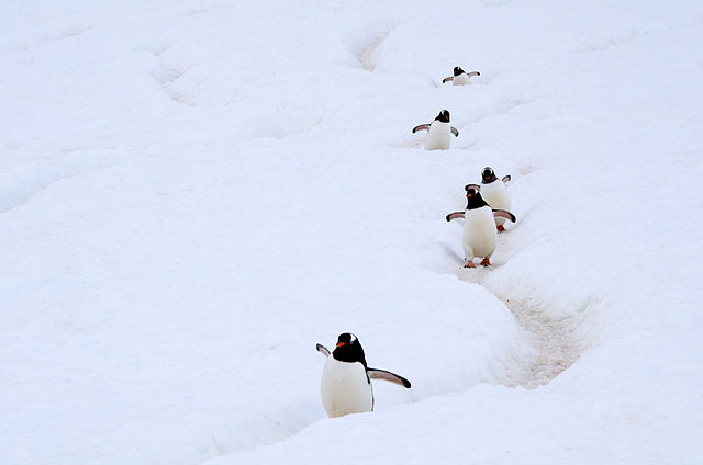
Who doesn’t like penguins? They have a quirky charm, and are an amazing demonstration of the power of evolution: they fly but only underwater, and are adapted to thrive in some of the harshest climates on Earth.
The {palmerpenguins} R package contains data collected at the Palmer Station on Anvers Island in the Antarctic. The data is measurement information about three different species of penguins, from three smaller islands in the area. You can find out more about the data in the package, as well as some examples of exploring and analyzing the data using R, here: https://allisonhorst.github.io/palmerpenguins/
![]()
Fixed-width files
This exercise in data import uses a modification of the data found in the {palmerpenguins} package—I have converted the data file to a fixed-width format. 1
This type of plain text file isn’t used as much as other types, but you may come across them in your data science journey.
One of the attributes of fixed-width files is that there are no delimiters as there are in file types such as CSV (Comma-Separated Value) and TSV (Tab-Separated Value) files. Instead, variables are assigned to specific columns in the file’s rows. This means that for very large files, reading the data can be accomplished more efficiently because there is no need to search for commas or other delimiters as every row is read. In addition, the challenge of embedded delimiters is eliminated, since there are none at all.
When computer memory was far more expensive than it is now, there was a cost incentive to create files that minimized the number of characters, including white space. This incentive was compounded when data was stored on punch cards, which had a physical constraint of an 80 character width; in that scenario, methods to eliminate any superfluous characters were sought. 2
Here in 2020, cheaper storage and efficient compression methods have meant that CSV files with unfixed variable lengths are more common, but in some big data applications, fixed-width files are still used.
Fixed-width penguins
The first 10 rows of the penguins_fwf.txt file look like this:
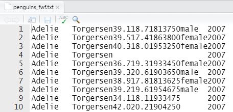
Note that the first row does not contain the variable names, but the first record—the observed characteristics of the first penguin in our dataset. This type of structure, with the variable names stored separately, is common in fixed-width files.
Also note that white space is at a minimum. For example, in the first records there are two blank spaces after the word “male” because “female” has two more letters (as is shown in the second record); the variable has to be wide enough to accommodate the value with the most characters. In data files where the creators are really serious about saving space, a variable like sex would be coded using a single digit (perhaps 1 = “female” and 2 = “male”, but be careful! 3), rather than the six characters required to spell out the words.
In the penguins_fwf.txt file there are 8 different variables, described in the table below:
| Variable | Width | Start position | End position |
|---|---|---|---|
| species | 9 | 1 | 9 |
| island | 9 | 10 | 18 |
| bill_length_mm | 4 | 19 | 22 |
| bill_depth_mm | 4 | 23 | 26 |
| flipper_length_mm | 3 | 27 | 29 |
| body_mass_g | 4 | 30 | 33 |
| sex | 6 | 34 | 39 |
| year | 4 | 40 | 43 |
This sort of detailed table is a common component in a data dictionary for a fixed-width file, and is an important element in programming the code to parse the file. In addition to providing vital information to the data user, developing this table also provides a double-check for the data preparer on the accuracy of the location specifications.
Importing fixed-width files with {readr}
The tidyverse package {readr}, part of the tidyverse family of R packages, provides a range of functions that make reading these files efficient.
The widths and variable names can be added as lists to the fwf_widths argument:
read_fwf("penguins_fwf.txt",
         fwf_widths(widths = c(9, 9, 4, 4, 3, 4, 6, 4),
                    col_names = c("species", "island", "bill_length_mm", "bill_depth_mm",
                      "flipper_length_mm", "body_mass_g", "sex", "year")))
# A tibble: 344 × 8
species island bill_length_mm bill_depth_mm flipper_length_mm body_mass_g
<chr> <chr> <dbl> <dbl> <dbl> <dbl>
1 Adelie Torgersen 39.1 18.7 181 3750
2 Adelie Torgersen 39.5 17.4 186 3800
3 Adelie Torgersen 40.3 18 195 3250
4 Adelie Torgersen NA NA NA NA
5 Adelie Torgersen 36.7 19.3 193 3450
6 Adelie Torgersen 39.3 20.6 190 3650
7 Adelie Torgersen 38.9 17.8 181 3625
8 Adelie Torgersen 39.2 19.6 195 4675
9 Adelie Torgersen 34.1 18.1 193 3475
10 Adelie Torgersen 42 20.2 190 4250
# ℹ 334 more rows
# ℹ 2 more variables: sex <chr>, year <dbl>A second option is to provide two lists of locations using fwf_positions(), the first with the start positions, and the second with the end positions. The first variable “species” starts at position 1 and ends at position 9, and the second variable “island” starts at 10 and ends at 18, and so on.
read_fwf("penguins_fwf.txt",
         fwf_positions(start = c(1, 10, 19, 23, 27, 30, 34, 40),
                       end = c(9, 18, 22, 26, 29, 33, 39, 43),
                       col_names = c("species", "island", "bill_length_mm", "bill_depth_mm",
                      "flipper_length_mm", "body_mass_g", "sex", "year")))
# A tibble: 344 × 8
species island bill_length_mm bill_depth_mm flipper_length_mm body_mass_g
<chr> <chr> <dbl> <dbl> <dbl> <dbl>
1 Adelie Torgersen 39.1 18.7 181 3750
2 Adelie Torgersen 39.5 17.4 186 3800
3 Adelie Torgersen 40.3 18 195 3250
4 Adelie Torgersen NA NA NA NA
5 Adelie Torgersen 36.7 19.3 193 3450
6 Adelie Torgersen 39.3 20.6 190 3650
7 Adelie Torgersen 38.9 17.8 181 3625
8 Adelie Torgersen 39.2 19.6 195 4675
9 Adelie Torgersen 34.1 18.1 193 3475
10 Adelie Torgersen 42 20.2 190 4250
# ℹ 334 more rows
# ℹ 2 more variables: sex <chr>, year <dbl>The third option, fwf_cols, is a syntactic variation on the second approach, with the same values but in a different order. This time, all of the relevant information about each variable is aggregated, with the name followed by the start and end locations.
read_fwf("penguins_fwf.txt",
         fwf_cols(species = c(1, 9),
                  island = c(10, 18),
                  bill_length_mm = c(19, 22),
                  bill_depth_mm = c(23, 26),
                  flipper_length_mm = c(27, 29),
                  body_mass_g = c(30, 33),
                  sex = c(34, 39),
                  year = c(40, 43)
         ))
# A tibble: 344 × 8
species island bill_length_mm bill_depth_mm flipper_length_mm body_mass_g
<chr> <chr> <dbl> <dbl> <dbl> <dbl>
1 Adelie Torgersen 39.1 18.7 181 3750
2 Adelie Torgersen 39.5 17.4 186 3800
3 Adelie Torgersen 40.3 18 195 3250
4 Adelie Torgersen NA NA NA NA
5 Adelie Torgersen 36.7 19.3 193 3450
6 Adelie Torgersen 39.3 20.6 190 3650
7 Adelie Torgersen 38.9 17.8 181 3625
8 Adelie Torgersen 39.2 19.6 195 4675
9 Adelie Torgersen 34.1 18.1 193 3475
10 Adelie Torgersen 42 20.2 190 4250
# ℹ 334 more rows
# ℹ 2 more variables: sex <chr>, year <dbl>And finally, {readr} provides a fourth way to specify the variables in a fixed-width file. Similar to the previous example, this variation has the name and the width values specified together.
# read
read_fwf("penguins_fwf.txt",
         fwf_cols(
           species = 9,
           island = 9,
           bill_length_mm = 4,
           bill_depth_mm = 4,
           flipper_length_mm = 3,
           body_mass_g = 4,
           sex = 6,
           year = 4
           )
         )
# A tibble: 344 × 8
species island bill_length_mm bill_depth_mm flipper_length_mm body_mass_g
<chr> <chr> <dbl> <dbl> <dbl> <dbl>
1 Adelie Torgersen 39.1 18.7 181 3750
2 Adelie Torgersen 39.5 17.4 186 3800
3 Adelie Torgersen 40.3 18 195 3250
4 Adelie Torgersen NA NA NA NA
5 Adelie Torgersen 36.7 19.3 193 3450
6 Adelie Torgersen 39.3 20.6 190 3650
7 Adelie Torgersen 38.9 17.8 181 3625
8 Adelie Torgersen 39.2 19.6 195 4675
9 Adelie Torgersen 34.1 18.1 193 3475
10 Adelie Torgersen 42 20.2 190 4250
# ℹ 334 more rows
# ℹ 2 more variables: sex <chr>, year <dbl>As with all of the functions in {readr}, we have the ability to specify the type of variables we want in our data in the script the reads the file. Heed the wisdom of Jenny Bryan:
My main import advice: use the arguments of your import function to get as far as you can, as fast as possible. Novice code often has a great deal of unnecessary post import fussing around. Read the docs for the import functions and take maximum advantage of the arguments to control the import. 4
Here’s the docs for the {readr} functions to “Read a fixed width file into a tibble”: https://readr.tidyverse.org/reference/read_fwf.html
An example: starting with the fwf_cols option we saw above, the code below uses col_types to specify “sex” as a factor, and “year” as an integer.
For this final version, I’ve used the kable() function from the {knitr} package to render the first 10 rows from the table.
# with column specification
penguins <-
read_fwf("penguins_fwf.txt",
         fwf_cols(
           species = 9,
                  island = 9,
                  bill_length_mm = 4,
                  bill_depth_mm = 4,
                  flipper_length_mm = 3,
                  body_mass_g = 4,
                  sex = 6,
                  year = 4
           ),
         col_types =
           cols(sex = col_factor(),
                year = col_integer())
         )

knitr::kable(head(penguins, n = 10), format = "html")| species | island | bill_length_mm | bill_depth_mm | flipper_length_mm | body_mass_g | sex | year |
|---|---|---|---|---|---|---|---|
| Adelie | Torgersen | 39.1 | 18.7 | 181 | 3750 | male | 2007 |
| Adelie | Torgersen | 39.5 | 17.4 | 186 | 3800 | female | 2007 |
| Adelie | Torgersen | 40.3 | 18.0 | 195 | 3250 | female | 2007 |
| Adelie | Torgersen | NA | NA | NA | NA | NA | 2007 |
| Adelie | Torgersen | 36.7 | 19.3 | 193 | 3450 | female | 2007 |
| Adelie | Torgersen | 39.3 | 20.6 | 190 | 3650 | male | 2007 |
| Adelie | Torgersen | 38.9 | 17.8 | 181 | 3625 | female | 2007 |
| Adelie | Torgersen | 39.2 | 19.6 | 195 | 4675 | male | 2007 |
| Adelie | Torgersen | 34.1 | 18.1 | 193 | 3475 | NA | 2007 |
| Adelie | Torgersen | 42.0 | 20.2 | 190 | 4250 | NA | 2007 |
-30-
Footnotes
You can download the fixed-width version of the palmerpenguins data file in both these locations: penguins_fwf.txt on this site or penguins_fwf.txt from google drive↩︎
Randall Munroe, Google’s Datacentres on Punch Cards↩︎
Boys will be boys: Data error prompts U-turn on study of sex differences in school—RetractionWatch.com↩︎
Jenny Bryan, STAT545, Chapter 9: Writing and reading files↩︎